Bayes vs Frequentists – An Empirical Test In Code

You and your friend are walking by a magic store and find a trick coin. You have no clue how biased the coin is, and decide that all possible levels of bias are equally likely. In order to estimate the level of bias, you toss it 14 times and end up with 10 heads.

Your friend is a compulsive gambler and wants to bet $10 that at least one of the next 2 flips will be tails. Should you take him on?

No really, should you take him on? This isn’t a philosophical, moral or “lateral thinking” question. This is a purely mathematical question. Given only the above explicitly stated assumptions and information, are the odds in your favor? Take a second to think about how you would solve this problem, in order to better appreciate the following discussion.

Frequentist Probability

When I pose this question to most people, their answer involves using frequentist probability.

You tossed the coin 14 times and got 10 heads. Therefore, the best estimate you have for the coin’s bias is 10/14. The odds of the next 2 coin tosses being heads, is simply 10/14 * 10/14, which is approximately 51%. The odds are in your favor, take the bet.

Spoiler alert: Despite the intuitive simplicity of this approach, it actually gives the wrong answer to the above problem!

Bayesian Statistics

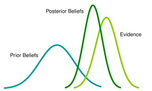
If you talk to statistics experts however, you’ll hear a completely different solution. One that uses Bayesian statistics. It works as follows:

You consider the universe of all possible coins, representing all different levels of bias. Let’s call this universe U. Within this universe, you consider the sub-universe of all coins/scenarios that will give you exactly 10 heads when tossed 14 times. Let’s call this S. And finally, within this sub-universe, you consider all possible outcomes that will give you 2 heads on the following 2 coin tosses. Let’s call this W. The probability of you winning the bet is now given by W / S.

Turns out the math for the above isn’t nearly as simple as the frequentist approach, but it can certainly be done. And the bayesian answer comes out to 48.5%. Your friend is smarter than he looks, don’t bet against him.

An Empirical Test

Well, you have 2 theories giving you diametrically opposite financial advice. In particular, the second theory involves complex mathematical techniques such as integrals that you don’t feel confident in correctly applying. What do you do next?

Luckily for us programmers, we can solve this problem with minimal mathematical training. All we need to do is run an empirical experiment … in code.

First, define a Coin class. Whenever an instance is constructed, it is seeded with a fixed and random amount of bias between 0 and 1 (as explicitly stated in the original problem). For example, a weight of 0.7 would mean that the coin is 70% likely to show heads, on each flip. We can use Java’s Random.nextDouble() in order to ensure that all levels of bias are equally likely. Ie, you’re just as likely to get a coin with a 10% bias, compared to an 80% bias.

Note: The above mirrors the originally stated assumption – “you have no clue how biased the coin is, and decide that all possible levels of bias are equally likely.” It is impossible to answer this problem without making an assumption of some kind. Hence why this was explicitly stated in the original problem statement. We will later discuss how different assumptions will lead to different results.

public static Coin createRandomCoin() {
  return new Coin(RNG.nextDouble());
}

private Coin(double weight) {
  this.weight = weight;
}

// Returns true for HEADS
public boolean flip() {
  return RNG.nextDouble() < weight;
}

We can also use the above flip method, in order to implement a simple helper method that will flip a given coin N times, and return the number of heads seen.

// Flip n times, and returns the number of heads
public int flip(int numFlips) {
  return (int) IntStream.range(0, numFlips)
  .mapToObj(i -> flip())
  .filter(isHeads -> isHeads)
  .count();
}

Next, we generate 10 million instances of the above coin, as a sample set for our empirical experiment.

Collection<Coin> betCoins = LongStream.range(0, 10000000)
  .mapToObj(i -> Coin.createRandomCoin())
  ...

We then flip each coin 14 times, and keep only those coins that produce exactly 10 heads. This gives us a representative sample of coins that led to the original problem statement.

Collection<Coin> betCoins = LongStream.range(0, 10000000)
  .mapToObj(i -> Coin.createRandomCoin())
  .filter(coin -> coin.flip(14) == 10)
  .collect(Collectors.toList());

And finally, now that we have recreated the original problem statement, we flip each of those coins 2 more times, and see how many produce 2 heads.

long numBetsWon = betCoins.stream()
  .filter(coin -> coin.flip(2) == 2)
  .count();

The fraction of bets that you would have won, is now easy to compute:

double fractionOfBetsWon = numBetsWon * 1.0 / betCoins.size();

The above empirical test has been coded up here, and here’s the result I see when running the experiment with a sample size of 10 million coins: 

48.56% of the time, you will get 2 heads on your 2 subsequent tosses.

Pretty damn close to the ~48.5% predicted by Bayesian statistics, and a resounding win over the frequentist prediction of 51%. You can see why Bayesian statistics is all the rage.

Alternative Facts

The above may seem like a thumping endorsement for bayesian statistics, but one open question still remains.

The above simulation was based on the premise that all levels of bias are equally likely. This was implemented by our createRandomCoin method, which uses Random.nextDouble, which in turn returns a random number between 0 and 1, where all possible values are equally likely. In Bayesian statistics, this is known as the prior.

In the absence of all information, the above premise is certainly a very reasonable starting point. But it isn’t the only one. One could argue that we should instead use a bell curve, so as to overweight the probability of more moderate amounts of bias, and underweight more extreme amounts of bias. Suppose we tweaked our code to use a bell curve instead:

public static Coin createRandomCoin() {
  return new Coin(getRandomSampleFromNormalDistribution());
}

private static double getRandomSampleFromNormalDistribution() {
  double percentile = RNG.nextDouble();
  double sample = new NormalDistribution(0.5, 0.2).inverseCumulativeProbability(percentile);
  if (sample < 0 || sample > 1) {
    return getRandomSampleFromNormalDistribution();
  } else {
    return sample;
  }
}

Our odds of winning now drops to ~42.4%. Even lower than before.

Conversely, one could also argue that we should use a U shaped probability distribution, that overweights more extreme levels of bias, and underweights moderate levels of bias – after all, we did find this coin next to a magic store. Suppose we tweaked our code to use this distribution instead:

public static Coin createRandomCoin() {
  return new Coin(getRandomSampleFromUDistribution());
}

private static double getRandomSampleFromUDistribution() {
  double normalSample = getRandomSampleFromNormalDistribution();
  if (normalSample < 0.5) {
    return 0.5 - normalSample;
  } else {
    double deltaFromMedian = normalSample - 0.5;
    return 1.0 - deltaFromMedian;
  }
}

Now our odds of winning have increased to ~57.9% instead! This analysis strongly recommends taking on the bet, even more so than the frequentist analysis.

At this point, we’ve seen three different priors produce three very different answers, ranging from 43% to 58%. In fact, you can derive any answer you want, by cherry-picking an extremely skewed prior.

Given this ambiguity, it is very tempting to just wipe the slate clean and go back to a simple frequentist approach. In fact, there even exists a probability distribution function that will lead to both bayesian and frequentist approaches producing the exact same result. Unfortunately, this frequentist approach also produces extremely bad results. For example, it would conclude a 100% certainty of your 3rd coin toss producing heads, just because your 1st and 2nd coin toss happened to be heads – a nonsensical conclusion that would lead to disaster if acted upon.

The silver lining is that as we increase the number of coin-flips, the different priors start converging. For instance, when flipping the coin 14 times, we have seen answers of 42.4%, 48.5% and 57.9% for the normal, uniform and U distributions. When we rerun the same simulation with 140 coin-flips and 100 heads, we instead see answers of about 49.6%, 50.6% and 51.8%. The prior is hugely influential when you have very few data points, but its effect is minimized as you collect more and more data points.

Given that choosing your prior is a subjective decision, there is bound to be endless controversy and debate around it. But hopefully the above simulation has demonstrated the methodology behind Bayesian statistics. And how we as developers can apply it to solve very tricky problems without any training in advanced mathematics.